Hypothesize Complexity with a Grammar

TASK #1 (8 steps): Make a ratio-complexity hypothesis.

A ratio-complexity hypothesis predicts how some ratios will be perceived as complex, unstable, or “unpulsed”, and others as simple, stable, and pulsed. In this task, you will look at a “radial” image of a limited set of ratios. Although many features of the image will not be explained here, you will begin to think intuitively about the factors that make a ratio like 7:2, or 9:4, more complex than ratios like 1:1 or 2:1.

1. Open Unpulser and choose File -> Open Project. Choose the project called “Project_Quickstart”, which can be found in the Unpulser directory you downloaded.

2. When you choose the project, a window called “Grammar: startup” opens.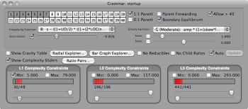

Click File -> Save Project As, give your project a memorable name, and save it to a folder that you won’t lose track of.

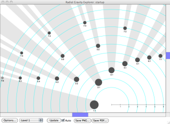
3. Click on the “Radial Explorer” Button, in the center-left of the “Grammar: startup” window. The radial window appears. If necessary, re-size the window and double-click on its image, to zoom in (& option-click to zoom out) and drag the image within the window, so that you can read the ratio labels. (The bottom and top halves of the circles are equivalent, so you can zoom in on one half or the other.)

This should help you to imagine complex ratios on outer circles, and simple ratios on inner circles.

4. In the upper-leftmost region of the Grammar window, note a grid containing the #s 1-40 in two rows, with the #s 1-7 darkened:

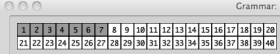
These represent available timespans for rhythms. Click numbers “8” and “9” to add those values to the available vocabulary. Notice the Radial Explorer updates automatically. Notice that large-sum ratios are on wider circles than smaller-sum ratios, and notice that only irreducible ratios are included. (If a large ratio is reducible, it is considered simple, and so it belongs on the circle associated with its reduced, smaller sum.)

5. In the center right of the Grammar window, find the “Gravity Function” menu. Beneath it is a slider called “Scale”.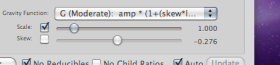

Click the check-mark in the box bedside it:

6. Experiment with the Gravity Function’s “Scale slider” and notice the Radial Window updating. When you increase the scale, ratio dots get bigger, and cast bigger shadows. When shadows “block” our view of a ratio further from the center, it is a hypothesis that the far-away ratio is indistinguishible from its nearby counterpart. This should suggest to you that unfamiliar ratios (the ones with large values) might be perceived within larger categories formed by more familiar ones (with smaller values). When you’ve experimented enough, click the scale value (shown to the right of the scale slider). A window opens, allowing you to enter a new value. Enter 1.5. (The default value is 1.)

7. Just below the timespan grid, find the “Irregularity Function” menu.

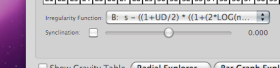Change the function from Z to B. Notice that in the Radial Explorer, all ratios that sum to prime numbers will stay where they are. The other (unprime) ratios will contract, to varying degrees, moving toward the center of the image. This assigns them a lesser “irregularity” value, and it means that rhythms with those ratios in them will be considered less complex than would otherwise have been the case.

8. Congratulations, you have a hypothesis. The image that you choose by adjusting these controls should be an image that reflect your best guess as to how one ratio might be perceived as more complex than another. To adjust your image further, experiment with different combinations of adjustments. You might also want to play with the “Synclination” slider (below the Irregularity function menu) by selecting it and micro-adjusting the difference between unprime and prime ratios. (The default value is zero.)

***

Now you might ask yourself: If you made experimental rhythms by connecting the timespans on the edges of your graph, one after the other, how complex, or “unpulsed”, would you guess them to be? What if you connected the timespans nearer the center of the graph? Try adjusting your settings (and your radial image) to produce different arrangements, and consider what they represent. (You’ll get to hear them in Task #2.)